
《Operating Systems: Three Easy Pieces》读书笔记(第 1-13 章)
闻名已久的操作系统著作,今日拜读一下。在线版本可以在这里找到,本文是第 1-13 章的笔记。内容基于自身情况记录,仅供参考,Dialogue 的相关章节已略过。
Chapter 2: Introduction to Operating Systems
- Operating System (aka virtual machine, supervisor, master control program) uses virtualization technique to provide a more easy-to-use layer (system calls -> standard library) for the above applications.
- CPU virtualization: turning a single CPU into a seemingly infinite number of CPUs and thus allowing many programs to seemingly run at once.
- Memory virtualization: each process accesses its own private virtual address space (VAS), which the OS somehow maps onto the physical memory of the machine.
- Brief history of the OS:
- Library: including commonly-used functions called by human operator.
- System call: adding user mode and kernel mode to provide protection for the OS. The idea here was to add a special pair of hardware instructions and hardware state to make the transition into the OS a more formal, controlled process.
- Multiprogramming: loading a number of jobs into memory and switch rapidly between them.
- Unix: leveraged by most of the OSes internally.
Chapter 4: The Abstraction - Process
- Mechanisms of CPU virtualization:
- Context switch: the ability to stop running one program and start running another.
- Scheduling policy: which decides how the processes should be switched.
- The constitution of a Process (PCB):
// A real case: xv6.
// Per-process state.
struct proc {
  uint sz;                     // Size of process memory (bytes).
  pde_t* pgdir;                // Page table.
  char *kstack;                // Bottom of kernel stack for this process.
  enum procstate state;        // Process state.
  int pid;                     // Process ID.
  struct proc *parent;         // Parent process.
  struct trapframe *tf;        // Trap frame for current syscall.
  struct context *context;     // swtch() here to run process.
  void *chan;                  // If non-zero, sleeping on chan.
  int killed;                  // If non-zero, have been killed.
  struct file *ofile[NOFILE];  // Open files.
  struct inode *cwd;           // Current directory.
  char name[16];               // Process name (debugging).
};
- The process can be described by its state:
- The contents of memory in its address space.
- The contents of CPU registers.
- The information about I/O.
- Three process states (at least, some may have Initial and Final states):
- Initial (optional): a process is just created.
- Running: a process is running on a processor.
- Ready: a process is ready to run but for some reason the OS has chosen not to run it at this given moment.
- Blocked (Waiting): a process has performed some kind of operation that makes it not ready to run until some other event takes place (e.g. waiting for IO request finished).
- Final / Zombie (optional): a process has exited but has not yet been cleaned up by OS, this is useful for examining the return code of the process.

Chapter 5: Interlude - Process API
- Process-related calls: the separation of fork() and exec() allows the shell to do a whole bunch of useful things rather easily.
- (POSIX.1) fork(): creating new process.
- This API creates an almost exact copy of the calling process as the basis for the created child process.
- Under Linux, fork() is implemented using copy-on-write pages, so the only penalty that it incurs is the time and memory required to duplicate the parent’s page tables, and to create a unique task structure for the child.
- (POSIX.1) wait() / waitpid(): waiting for children processes to finish.
- (POSIX.1) exec(): replacing the current process image with a new process image. It loads code and static data from the specified executable and overwrites its current code segment with it, the heap and stack and other parts of the memory space are re-initialized. This API never returns.
- (POSIX.1) kill(): sending signals to a process.
- (POSIX.1) signal(): setting the way of disposition for specific signal.
- A similar implementation of redirection:
// rough-redirection.c
// prompt> wc rough-redirection.c > redirection.output.txt
#include <stdio.h>
#include <stdlib.h>
#include <unistd.h>
#include <string.h>
#include <fcntl.h>
#include <sys/wait.h>
int main(int argc, char* argv[]) {
  int rc = fork();
  if (rc < 0) {
    fprintf(stderr, "fork failed.\n");
    exit(1);
  } else if (rc == 0) {  // The child process.
    // UNIX systems start looking for free file descriptors at zero, -
    // so here we close STDOUT(0) and open the target one.
    close(STDOUT_FILENO);  // Close standard output.
    open("redirection.output", O_CREAT | O_WRONLY | O_TRUNC, S_IRWXU);  // Open the file instead.
    char* wc = strdup("wc");
    char* args[] = { wc, strdup("rough-redirection.c"), NULL };
    execvp(wc, args);
  } else {  // The main process.
    int rc_wait = wait(NULL);
  }
  return 0;
}
- Unix pipes are implemented with the system call - pipe().
- The separation of fork() and exec() enables features like: input/output redirection, pipes, and other cool features, all without changing anything about the programs being run.
- C Standard Library V.S. Standard C Library: there are some interfaces that are not part of the C Standard, but part of the Standard C Library implementation (e.g. glic), for example the APIs defined in unistd.h that exposed the access to POSIX OS APIs.
Chapter 6: Mechanism - Limited Direct Execution
- Limited direct execution: run the program directly on the CPU with some controls.
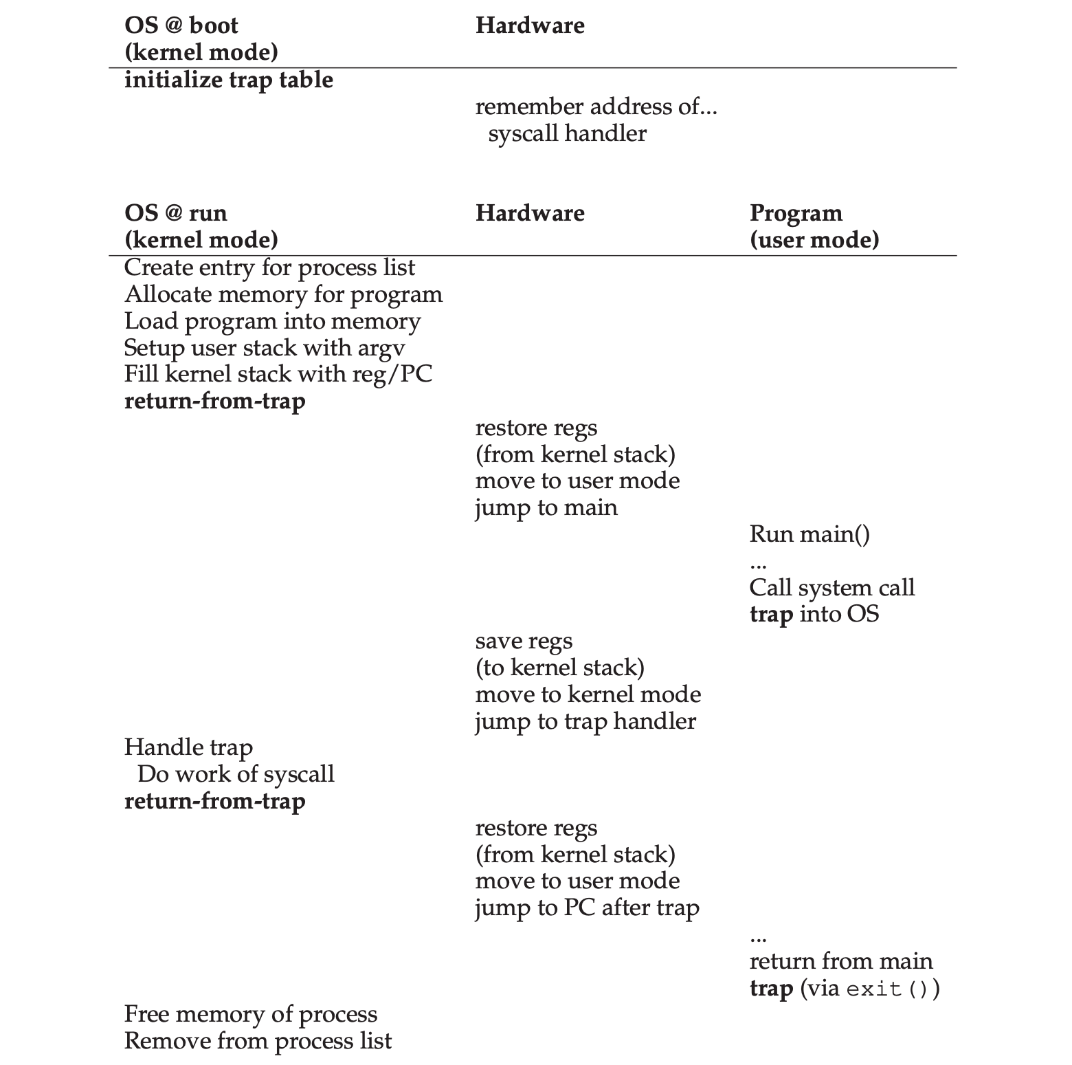
- Each process has a “kernel stack“ area to save and restore the user registers during context-switching.
- Two modes of execution: user mode (restricted) & kernel mode (privileged).
- OS could regains control of the CPU by either:
- Cooperative approach: by waiting for a system call or an illegal operation of some kind to take place, the OS then can take over the CPU.
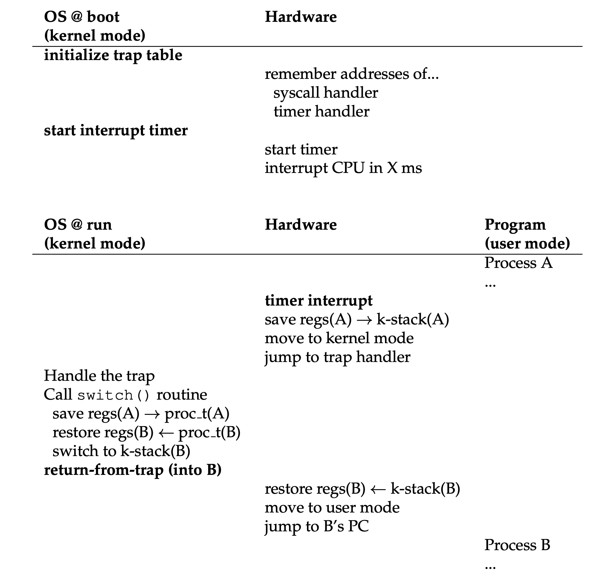
- Non-Cooperative approach: setup a programmed timer device to raise an interrupt every so many milliseconds. When the interrupt is raised, the currently running process is halted, and a pre-configured interrupt handler in the OS runs. At this point, the OS has regained control of the CPU.
- Context switch: in xv6, context switching only involves program observable registers, and for other registers and data like below, they all would be updated by the kernel. Please note that the cost is not only from the switch of registers but also the flush of CPU states (TLB, caches, branch predictions, etc).
- cr3: page directory base register.
- tr: task register.
- ss0-ss3: contains the stack segment selector for different privileges.
- rsp0-rsp3: contains the stack top selector for different privileges.
The rough implementation of the context-switch logic:
# C definition.
struct context {
  uint edi;
  uint esi;
  uint ebx;
  uint ebp;
  uint eip;
};

# Context switch                                            |----------------|  (after "pushl %edi")
#                                                           | ptr_new (%edx) | --> |  struct context   |
#   void swtch(struct context **old, struct context *new);  | ptr_old (%eax) | --> | *(struct context) | --> | struct context |
#                                                           |      %eip      |
# Save the current registers on the stack, creating         |      %ebp      |
# a struct context, and save its address in *old.           |      %ebx      |
# Switch stacks to new and pop previously-saved registers.  |      %esi      |
#                                                           |      %edi      |
#                                                           |----------------| <- %esp
# Assembly code:

.globl swtch
swtch:
  movl 4(%esp), %eax  # old ptr.
  movl 8(%esp), %edx  # new ptr.

  # Save old callee-saved registers, the value of %eip is already on the stack.
  pushl %ebp
  pushl %ebx
  pushl %esi
  pushl %edi

  # Switch stacks.
  movl %esp, (%eax)  # Save new address to *old.
  movl %edx, %esp

  # Load new callee-saved registers.
  popl %edi
  popl %esi
  popl %ebx
  popl %ebp
  ret  # Will pop %eip direclty after return.
- Limited direct execution with timer interruption:
Chapter 7: Scheduling - Introduction
- Scheduling metrics (below two are mutually exclusive):
- Turnaround Time: Tturnaround = Tcompletion - Tarrival.
- Response Time: Tresponse = Tfirstrun - Tarrival.
- CPU scheduling algorithms:
- FIFO (non-preemptive): serve by their sequence, but may incur “convoy effect“ (a number of relatively-short potential consumers of a resource get queued behind a heavyweight resource consumer).
- SJF (Shortest Job First, non-preemptive): run and complete the shortest job first, then the next shortest, and so on. This approach may also incur “convoy effect“ issue if a long task comes first along with a short task coming shortly.
- PSJF (Preemptive Shortest Job First, preemptive): based on SJF, job can preempt the existing running jobs via context-switching.
- RR (Round-Robin, preemptive): runs a job for a time slice (aka scheduling quantum, must be a multiple of the timer-interrupt period) and then switches to the next job in the run queue. The length of the time slice is critical (response time V.S. context-switching penalty).
An inherent trade-off on scheduling: if we want to be unfair, we can run shorter jobs to completion, but at the cost of response time; if we instead value fairness, response time is lowered, but at the cost of turnaround time.
An example of PSJF with I/O operations considered:
- Task A: CPU - 50ms, runs for 10 ms and then issues an I/O request which takes 10ms for each.
- Task B: CPU - 50ms, no I/O request.

Chapter 8: Scheduling - The Multi-Level Feedback Queue
- MLFQ (Multi-Level Feedback Queue):
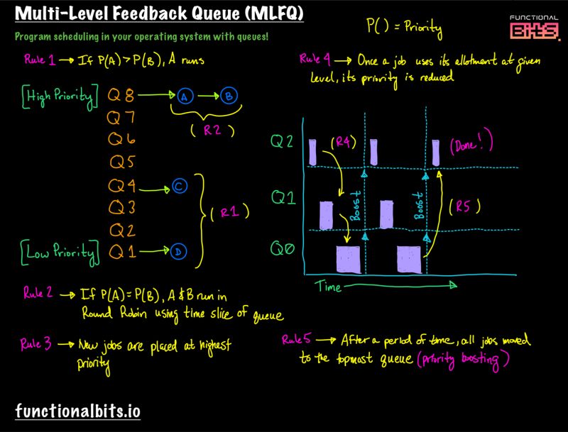
- It has a number of distinct queues, each assigned a different priority level with different time slice (the higher the shorter).
- It uses priorities to decide which job should run at a given time: a job with higher priority (i.e., a job on a higher queue) is chosen to run.
- Rule 1: if Priority(A) > Priority(B), A runs (B doesn’t).
- Rule 2: if Priority(A) = Priority(B), A & B run in round-robin fashion using the time slice (quantum length) of the given queue.
- Rule 3: when a job enters the system, it is placed at the highest priority (the topmost queue).
- Rule 4: once a job uses up its time allotment (the amount of time a job can spend at a given priority level) at a given level (regardless of how many times it has given up the CPU), its priority is reduced (i.e., it moves down one queue).
- Rule 5 (avoid starvation): after some time period S, move all the jobs in the system to the topmost queue.
- Types of workload need to consider:
- The interactive jobs that are short-running which may frequently relinquish the CPU.
- The longer-running “CPU-bound” jobs that need a lot of CPU time but where response time isn’t important.
- Some voo-doo constants need to consider:
- How many queues? 60.
- How big should the time slice be per queue? 20ms (highest) -> hundred ms (lowest).
- How often should priority be boosted? 1s or so.
- Other algorithm variants:
- Use mathematical formulae to calculate the priority level of a job, basing it on how much CPU the process has used.
- Reserve the highest priority levels for operating system work.
- Allow some user advice to help set priorities via CLI, like
nice.
- Learn from history based on the basic principles:
- I/O intensive - hight priority.
- CPU intensive - low priority.
Chapter 9: Scheduling - Proportional Share
- Proportional-share (fair-share) scheduler: a scheduler that guarantees that each job could obtain a certain percentage of CPU time.
- Lottery scheduling: every so often, hold a “lottery” (a random number) to determine which process should get to run next. The longer these jobs complete, the more likely they are to achieve the desired percentages.

- Basic steps:
- (optional) Make the process list in a sorted descending order based on the ticket number.
- Pick a random number (winner) from the total number of tickets.
- Traverse the list, adding each ticket value to the
counteruntil the value exceeds winner. - Then, the current list element is the winner.
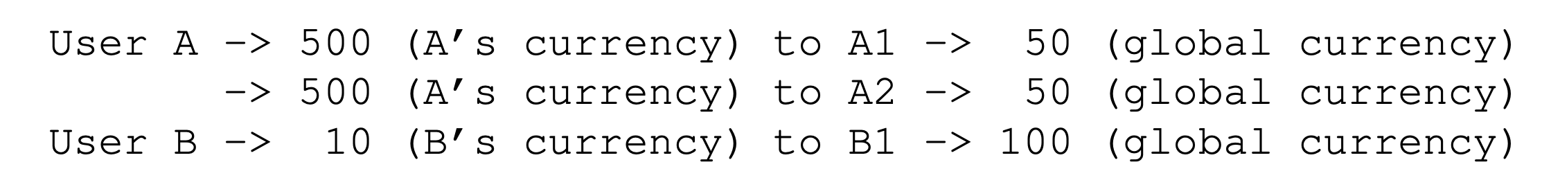
- Ticket currency: it allows a user with a set of tickets to allocate tickets among their own jobs in whatever currency they would like.
- Ticket transfer: a process can temporarily hand off its tickets to another process.
- Ticket inflation: a process can temporarily raise or lower the number of tickets it owns, tis can be applied in an environment where a group of processes trust one another.
- Problem: how to assign ticket to each process?
- Stride scheduling: at any given time, pick the process to run that has the lowest pass value so far; when you run a process, increment its pass counter by its stride.
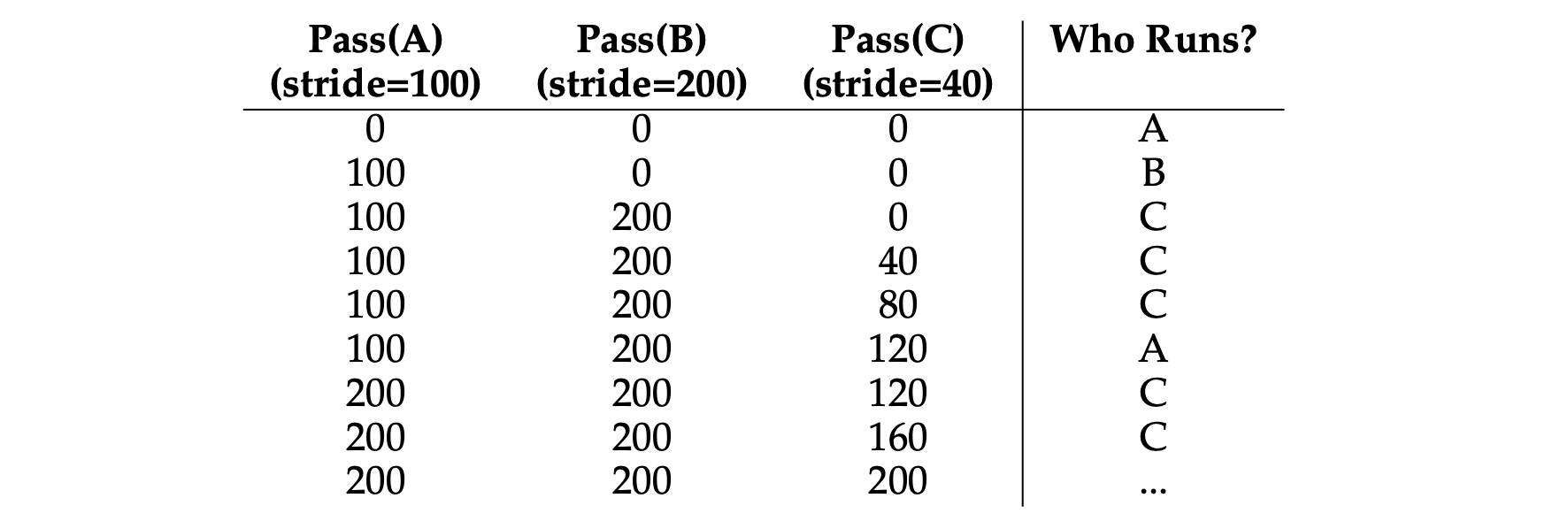
- Each job in the system has a stride, which is inverse in proportion to the number of tickets it has (a large number / #tickets).
- Problem: how to treat new processes for their initial pass?
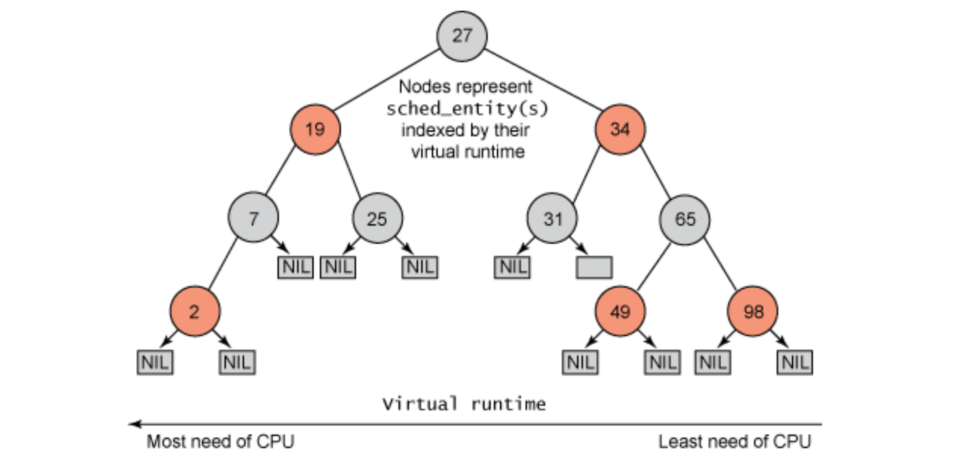
- CFS (Completely Fair Scheduler): CFS is being used inside Linux kernel, based on counting-based technique known as virtual runtime (vruntime), each process’s vruntime increases at the same rate, in proportion with physical (real) time. When a scheduling decision occurs, it will pick the process with the lowest vruntime to run next. It uses the value “sched_latency“ (usually 48ms) to determine how long one process should run before considering a switch. CFS divides this value by the number (n) of processes running on the CPU to determine the time slice for a process. CFS adds another parameter, “min_granularity“, which is usually set to a value like 6ms as the minimum time slice. CFS utilizes a periodic timer interrupt, it goes off frequently (e.g., every 1 ms), giving CFS a chance to wake up and determine if the current job has reached the end of its run. CFS keeps running processes in a red-black tree for a better search and insertion. Processes are ordered in the tree by vruntime, and most operations (such as insertion and deletion) are logarithmic in time. CFS sets the vruntime for the newly inserted job (ready) to the minimum value found in the RB tree.
Chapter 10: Multiprocessor Scheduling (Advanced)
- The issues may occur for multiple CPUs:
- Cache coherence: a running program has the correct latest data on CPU 1 but not CPU 2 due to the old data retrieved from main memory after scheduling. This issue could be solved by bus snooping - each cache pays attention to memory updates by observing the bus that connects them to main memory. When a CPU then sees an update for a data item it holds in its cache, it will notice the change and either invalidate its copy (i.e., remove it from its own cache) or update it (i.e., put the new value into its cache too).
- Concurrency: synchronization, and as the number of CPUs grows, access to a synchronized (with locks) shared data structure becomes quite slow.
- Cache affinity: the states of the running process are not reused after the CPU scheduling.
- SQMS (Single-Queue Multiprocessor Scheduling): putting all jobs that need to be scheduled into a single queue, but it does not scale well (due to synchronization overheads), and it does not readily preserve cache affinity.
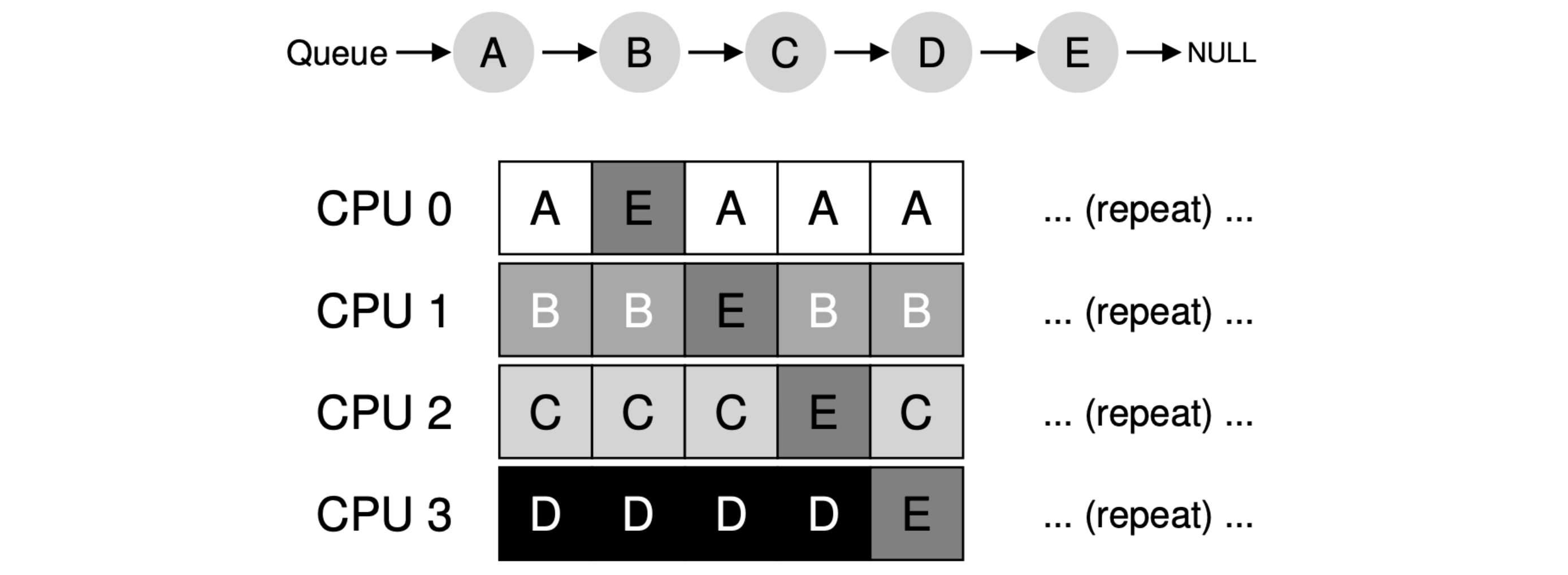
- How to keep load cache affinity? A: Most SQMS schedulers include some kind of affinity mechanism to try to make it more likely that process will continue to run on the same CPU if possible (like above, job E will be migrating from CPU to CPU).
- MQMS (Multi-Queue Multiprocessor Scheduling): based on SQMS, using multiple queues, one per CPU. When a job enters the system, it is placed on exactly one scheduling queue, according to some heuristic (e.g., random, or picking one with fewer jobs than others). Then it is scheduled essentially independently, thus avoiding the problems of information sharing and synchronization found in the single-queue approach.
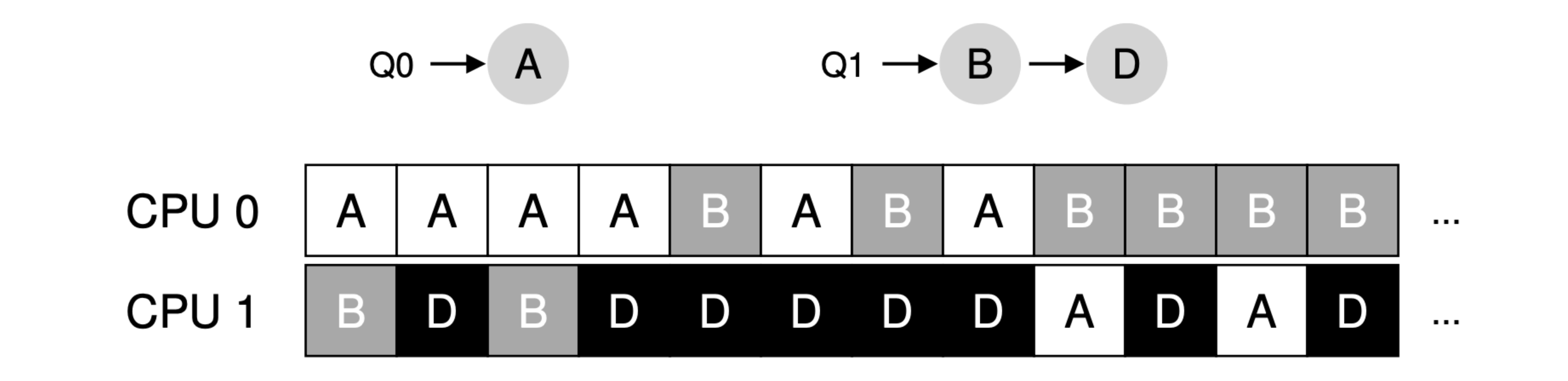
- How to solve load imbalance? A: With a work-stealing approach, a (source) queue that is low on jobs will occasionally peek at another (target) queue, to see how full it is. If the target queue is (notably) more full than the source queue, the source will “steal” one or more jobs from the target to help balance load.
- Linux multiprocessor schedulers:
- O(1): a priority-based scheduler (similar to the MLFQ), changing a process’s priority over time and then scheduling those with highest priority in order to meet various scheduling objectives; interactivity is a particular focus.
- CFS: a deterministic proportional-share approach.
- BFS: a single-queue and proportional-share approach, based on a more complicated scheme known as Earliest Eligible Virtual Deadline First (EEVDF).
Chapter 13: The Abstraction - Address Spaces
- Any address you can see as a programmer of a user-level program is a virtual address, only the OS (and the hardware) knows the real truth of the physical address.
评论 | Comments